NEATBird: Teaching Flappy Bird to Evolve on the GPU

Darwin, but the birds are JSON

The idea of teaching neural networks to reproduce with enough JSON did not come to me in a dream. It arrived by email, in the general vicinity of a take-home assignment for a job I did not get.

The idea stuck anyway. I wanted to point the same machinery at a completely different problem and see whether I understood it well enough to rebuild it myself.

The foundation is NeuroEvolution of Augmenting Topologies, or NEAT, introduced by Kenneth O. Stanley and Risto Miikkulainen in their 2002 paper, Evolving Neural Networks through Augmenting Topologies.

Normal neuroevolution can start with one fixed network shape and use a genetic algorithm to search for good weights. NEAT evolves the shape too. A genome can gain connections, split a connection with a new node, cross over with another genome, and become more complex only when that structure survives selection.

The original paper solved three awkward problems that appear as soon as neural networks stop having one fixed layout:

1. Historical markings make crossover meaningful. Every structural mutation receives an innovation number. When two differently shaped genomes reproduce, matching innovation numbers identify homologous genes. The algorithm does not need to stare at two graphs and hope node 17 means the same thing in both.
2. Speciation protects new structure. A fresh node or connection may initially make a network worse before its weights adapt. Similar genomes compete inside species, which gives structural experiments time to become useful instead of being deleted after one bad episode.
3. Networks start minimal and complexify. NEAT begins with the smallest useful topology. It adds structure as the task demands it, rather than starting with a giant random graph and asking evolution to perform garbage collection.

Canonical NEAT chooses matching genes randomly, takes disjoint and excess genes from the fitter parent, and can inherit unilateral genes randomly when fitness is equal. NEATBird follows Ha’s variant instead: matching columns can supply either parent’s weight, while the child copies the union of genes owned by only one parent.

The original NEAT method evolves both topology and weights through genetic operations. It can also support recurrent connections. My implementation keeps the historical markings, structural mutations, crossover, compatibility distance, and gradual complexification, but restricts every phenotype to a feed-forward DAG.

NEAT tracks ancestry so differently shaped networks can inherit useful structure without crossover turning their children into abstract art.

Backprop NEAT: the garage-metal original

The second foundation is David Ha’s 2016 work, Neural Network Evolution Playground with Backprop NEAT and its open-source implementation, hardmaru/backprop-neat-js.

Ha’s experiment gave NEAT one job and backpropagation another:

NEAT -> discover network structure
backpropagation -> optimize weights inside that structure

His JavaScript playground evolved arbitrary computational graphs for classification tasks inspired by TensorFlow Playground. The networks could discover heterogeneous operators such as sin, gaussian, square, multiply, and add instead of using one activation across a tidy stack of layers. recurrent.js handled forward and backward passes through the evolved graphs.

The work also replaced NEAT’s usual species assignment with five K-medoids clusters, kept a hall of fame, sampled extinction with a 50 percent probability, and penalized networks for excess connections. Ha used the clusters as a diversity heuristic. Canonical NEAT uses speciation with explicit fitness sharing. In Ha’s own analogy, deep learning researchers were pop idols while evolutionary-computing researchers were obscure garage metal bands. NEATBird is a GPU-heavy cover arrangement released ten years later.

NEATBird directly adapts those ideas and constants. The five clusters, activation palette, add-node and add-connection rates, per-gene weight mutation, extinction behavior, innovation-aligned crossover, and connection penalty all come from Ha’s implementation.

Ha trained on fixed labeled datasets with supervised logistic-regression loss. Flappy Bird gives actions and rewards rather than a correct label for every frame, so I use REINFORCE. Ha allowed recurrent loops; I validate every phenotype as a feed-forward DAG. recurrent.js ran his numerical engine. Mine compiles packed edge vectors into JAX, batches matching topologies with vmap, and runs game episodes with lax.scan. I also added deterministic game schedules, paired pre/post-update scoring, harmful-update rollback, portable checkpoints, and separate JAX and Pygame engines.

The lineage is:

Stanley and Miikkulainen's NEAT
  -> David Ha's Backprop NEAT
  -> feed-forward JAX Backprop NEAT for Flappy Bird

If the interesting part here is evolving small, strange computational graphs instead of another rectangular tower of ReLUs, read the original NEAT paper and Ha’s article first. I changed the venue from a classification playground to an airborne failure-analysis laboratory.

My Flappy Bird game can’t possibly be this easy!

I wanted to train a neural network to play Flappy Bird.

This is normally a solved afternoon project. Download neat-python, copy the classic Tech With Tim tutorial, leave it running for a while, and watch a tiny bird develop better survival instincts than most protagonists in a Key visual novel.

I took the longer route: building the genome format, innovation tracking, graph mutations, crossover, clustering, feed-forward compiler, policy-gradient optimizer, checkpoint format, vectorized game engine, and SVG renderer myself. Well, I actually just asked Claude to make no mistakes. The final trainer combines NEAT-style evolution with REINFORCE updates in JAX. Python evolves the graph. JAX trains its weights and simulates the flock. Pygame remains around for replay because I am still not fluent in clanker (all float values).

The first version worked almost offensively well. A three-connection linear policy reached 1,000 points on four seeds. It flew for 75,020 frames each time and stopped only because I told the episode that 1,000 points was enough.

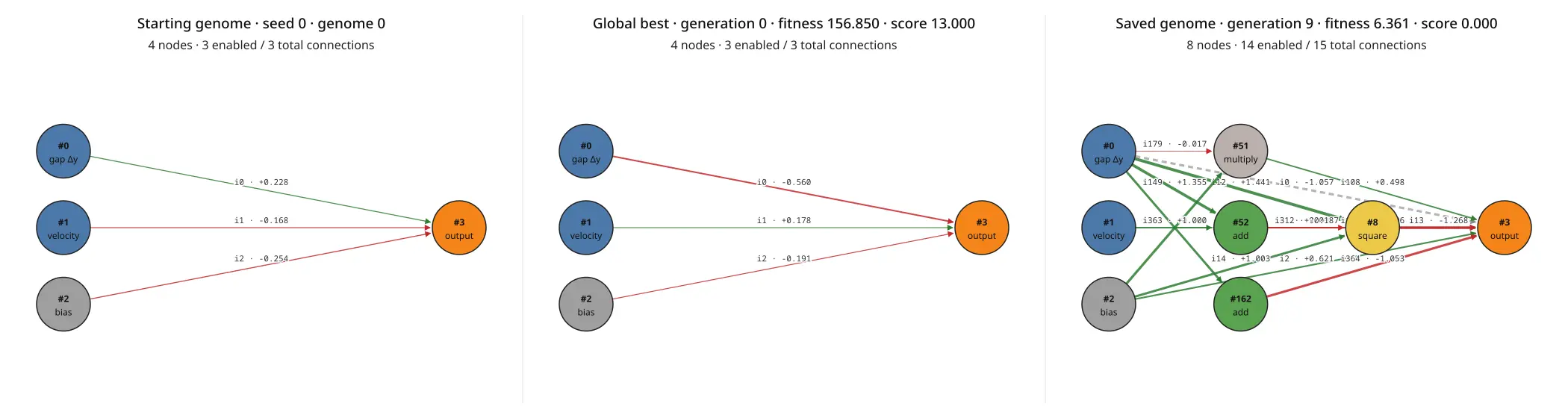The fixed-gap prototype. Evolution produced larger graphs, but the tiny linear champion had already solved the assignment.

The tutorial level was lying to me

Classic Flappy Bird NEAT agents usually receive two useful values:

1. vertical distance to the next gap;
2. current vertical movement.

The gap is always the same size. Its vertical position changes, but the safe action is close to a fixed threshold: flap when the bird is sufficiently below the center. A linear policy can do this. Mine did it in generation 0.

That is a nice demo of the trainer and a bad demo of topology evolution. The population could grow hidden nodes with sigmoid, tanh, relu, gaussian, sin, abs, multiply, square, and add, but complexity was mostly decorative. Basically, the funny guy mogging on the bodybuilder in social occasions.

I changed the task so a weighted sum had more to contend with.

Each pipe now gets a gap from 130 to 260 pixels. Gap centers alternate between lower and upper bands. The bird receives five observations:

current gap center - bird y-position
vertical displacement
current gap size
next gap center - bird y-position
current pipe x - bird x

Every value is normalized. The current gap size changes how much error is safe. The next center changes whether the bird should spend the current gap high or low before the next climb. Those interactions make products between inputs useful. The old two-input fixed threshold no longer has enough information.

Those interactions gave nonlinear graph structure something useful to model instead of drawing it for the README. I did not run a fixed-MLP baseline, so the champion’s eventual hidden node does not establish that topology evolution was necessary.

It also made every weakness in the trainer visible at once. The E2E test passed; the real user immediately flew into a pipe.

The weights begin their training arc

Evolution decides which wires exist; gradient descent tunes them. I wanted both.

Each NEAT genome owns node IDs and connection genes. A process-wide innovation store gives matching structural mutations stable innovation numbers so crossover can align them later.

The starting genome connects every input and one bias directly to one linear output. Children can:

• split a connection with a new hidden node;
• add an acyclic connection;
• perturb connection weights;
• inherit matching and unilateral genes from two parents.

Every graph remains a feed-forward DAG. A mutation that would create a cycle is rejected. Crossover keeps a cycle-producing inherited gene but disables it. Loaded checkpoints go through the same validation, because “the JSON said it was fine” is not a graph invariant.

The population is divided into five PAM k-medoids clusters using a NEAT-style compatibility distance. PAM encourages structurally different genomes to reproduce in separate clusters; it is not canonical NEAT speciation with explicit fitness sharing. Think Ave Mujica, except membership is decided by excess genes, disjoint genes, and weight differences, and the worst group has a 50 percent chance of being replaced by children from the best one. On reflection, this may still be Ave Mujica.

For each generation, the trainer:

reproduces genomes
  -> injects hall-of-fame and cluster elites
  -> groups matching topologies
  -> runs stochastic policy-gradient episodes
  -> applies RMSProp weight updates
  -> scores before and after on the same layouts
  -> rolls back harmful updates
  -> clusters the population again
  -> writes JSON checkpoints

The rollback matters. REINFORCE is noisy. If a candidate gets worse on the fixed selection/rollback layouts after four policy-gradient cycles, its weights and RMSProp cache return to their previous state. Evolution gets the improved candidate or the original one, not the version that had a bad afternoon.

Fitness also includes a connection penalty. More edges must earn their rent. If two genomes receive the same game return, the smaller graph wins.

Birds of a feather vmap together

The original Pygame state machine is useful for rendering and pixel-perfect collision masks. Evaluating 100 birds across many generations and policy-gradient cycles needed a second game engine in JAX. The held-out checkpoint evaluator uses this JAX engine too.

Both engines use the same bird motion, pipe motion, observation order, reward order, death conditions, and seeded pipe schedule. Their collision implementations differ: Pygame rounds the bird y-position and uses sprite masks, while JAX uses axis-aligned bounding boxes around the 68 by 48 pixel bird image. The box is slightly more conservative, so replay can differ by a pixel or two. Same manga, different key animation.

A training episode is one jax.lax.scan over a fixed number of frames. Birds are lanes in arrays. jax.vmap evaluates policies over the population. Genomes with the same reachable topology share compiled functions and run together.

The graph itself stays on the Python host. The compiler turns an acyclic genome into:

• a stable topological schedule;
• static source and destination arrays;
• activation codes;
• an innovation-ordered vector of enabled weights.

Only that packed weight vector enters automatic differentiation. I could have used a dense node-by-node weight matrix, but NEAT graphs are sparse and hidden nodes can multiply inputs or apply different activations. A dense matrix would mostly store zeros while the forward pass still followed graph order. The packed vector stores one value per enabled edge and gives gradients back in the exact order needed for checkpoint writeback.

Topology signatures do not include numeric weights. Change a weight and the compiled program is reused. Change reachable graph structure and JAX compiles a new one.

Static shapes are the price of making this fast. Population batches keep a fixed width. Episodes always scan max_frames steps. Dead birds become frozen lanes rather than shortening the loop. This is excellent for XLA and, as I eventually learned, capable of hiding a death just beyond the edge of the universe.

The bird practiced on one layout and was selected on another

After randomizing the pipes, the default run plateaued at two points. Generation 29 had the best candidate. Generation 49 still had the same best candidate. Most policy-gradient rounds printed something close to:

accepted=2 reverted=98

Ninety-eight birds would learn something and immediately have it taken away by the rollback gate.

My first suspect was network size. The gradients and selection logic were looking at different worlds.

Selection and rollback used:

seed + 9000
seed + 9001
seed + 9002

Policy-gradient rollouts used:

seed + generation * 10000 + cycle

The three selection layouts were optimization data: update acceptance, fitness, clustering, archives, and champion selection all depended on them. The candidate practiced on one layout, then rollback and evolutionary selection scored it on three others. The two optimization signals disagreed.

I added two optional controls:

--eval-seeds 0
--pg-seed 0

The flag name remains --eval-seeds, but its layouts perform selection and rollback. The defaults still support varying optimization layouts. Fixed-seed mode lets the gradient and the selection score refer to the same level while debugging. It is the machine-learning equivalent of checking whether the student can solve the worksheet before changing every question.

The next run improved from two pipes to 13 inside the 1,000-frame training window. A longer replay reached pipe 17 and died at frame 1,362.

The improvement came with a new bug wearing a different hat.

The same trainer before and after the seed fix: two pipes on the left, seventeen on the right.

The bird died after the credits

Training stopped after 1,000 frames. If a bird was alive at frame 1,000, the JAX scan ended and the candidate received no information about what happened next.

The 13-point champion was not “done” at the frame cap. It continued through four more pipes and died at 1,362. The failure was real, repeatable, and completely invisible to training.

I increased the window to 3,000 frames, so the trainer could see the death. It still could not get past pipe 17.

Two different champions reached the same place. One had 13 connections. The other had 14. Both died at the byte-identical frame 1,362. The score stayed at 17 from generation 33 through generation 49, with the failure inside the training horizon, and neither evolution nor gradient descent found a route through it.

The network was no longer a convincing suspect. I inspected the level.

I generated a pathological Touhou pattern

Around the death, seed 0 produced this sequence:

Pipe	Gap top	Gap size	Center	Band
16	59	196	157	Low
17	389	133	456	High
18	149	232	265	Low

The bird had to move roughly 298 pixels from a low center into a 133-pixel gap. The sprite is 48 pixels tall, leaving about 85 pixels of vertical slack. Flappy Bird movement is not continuous control. A flap resets vertical velocity, and frame updates quantize the resulting altitude. The tested controllers could undershoot or overshoot, and two independently trained networks died at the same frame.

The matching deaths made the transition look pathological. Without an exhaustive reachability search in either the Pygame mask engine or the JAX AABB engine, I could not establish whether any action sequence could clear it.

For consecutive gap centers separated by (d) pixels, I added a minimum target width:

gap >= min(260, ceil(120 + 0.15 * d))

The schedule first samples a gap from 130 through 260. Large vertical jumps widen a smaller target gap. If resampling the gap position still cannot satisfy the floor, the schedule uses the 260-pixel maximum.

I tuned the constants by playing candidate schedules through the Pygame physics with a heuristic controller. The jump-scaled floor made the observed transition less pathological, but I did not test every generated transition for reachability.

39 pipes in class, 66 after school

Run 4 used seed 0 for policy-gradient trajectories, rollback decisions, evolutionary fitness, and champion selection. With a 3,000-frame horizon and the repaired schedule, the best genome appeared in generation 9.

It had eight nodes and eight connection genes, seven of them enabled. Inside training, it cleared all 39 pipes available before the frame cap. In a longer replay on the same seed-0 schedule, it reached 66 pipes and died at frame 4,972.

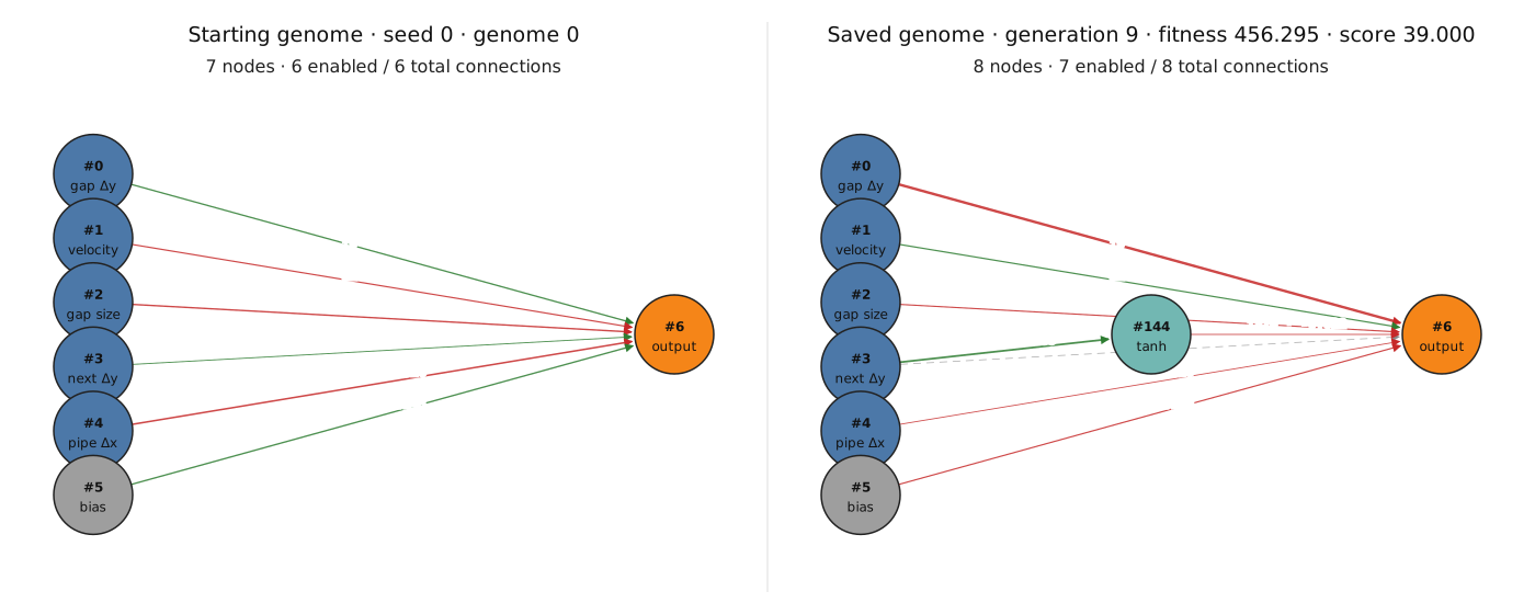
The repaired-schedule champion adds one hidden tanh node. Its eighth connection gene remains disabled and appears as a dashed edge.

Generation 9 clears 66 pipes. The animation samples every twentieth game frame so this page does not become a 75,000-frame hostage situation.

The full sequence looked like this:

Run	Schedule	Training window	Score seen in training	True replay death
1	Original randomized	1,000	2	About frame 214
2	Original randomized, fixed seed	1,000	13	17 pipes at frame 1,362
3	Original randomized, fixed seed	3,000	17	17 pipes at frame 1,362
4	Repaired randomized, fixed seed	3,000	39	66 pipes at frame 4,972

The repaired schedule satisfies the gap-floor heuristic near the final death. Pipes 40 onward are an unseen suffix of the seed-0 schedule, so the 66-pipe replay measures temporal extrapolation. Cross-schedule generalization required a separate held-out test.

I therefore ran the saved champion through the JAX AABB engine on a predeclared held-out range of 100 schedules:

uv run python tools/evaluate_champion.py \
  --genome checkpoints_fixed/best_genome.json \
  --seed-start 1000000 \
  --seed-stop 1000099 \
  --max-frames 5000

The model was checkpoints_fixed/best_genome.json. Its optimization schedule was seed 0. The test range was 1,000,000–1,000,099.

Metric	Result
Mean pipes	20.1
Median pipes	13.0
P10	0.0
P90	60.3
Minimum	0
Survived 5,000 frames	8%

These results measure held-out performance across schedules from the repaired generator. Reachability across every possible generated transition remains untested.

A bounded lax.while_loop could remove trailing iterations after the final lane dies. It would still process every fixed-width lane while any lane lives, and it would need fixed-shape trajectory buffers and masks. That optimization is viable here because policy-gradient code materializes trajectories before automatic differentiation; it would not remove the frame cap or make indefinite play a proven outcome.

Final thoughts

NEATBird started as “I want to train a neural network to play Flappy Bird” and became a disciplinary hearing for the bird, the teacher, the exam, and the laws of physics.

The champion cleared 66 pipes on its favorite level, averaged 20.1 on 100 strangers, and survived all 5,000 frames eight times. It has the energy of a gifted child who memorized one Mario Kart track. I will take it.

I still owe it a proper baseline and more runs, which is a dignified way of saying I need to kill more birds under controlled conditions. For now, I have a tiny evolved graph, a GPU full of frozen birds, and a benchmark that lies less than it used to. That is enough dead birds for one blog post.

Cheers!